13.021 – Marine Hydrodynamics

Lecture 24C – Lifting Surfaces

Introduction

Lifting surfaces in marine hydrodynamics typically have many applications such as hydrofoils, keels, rudders, propeller blades and yacht sails. A lifting surface is a thin streamlined body that moves in a fluid at a small angle of attack with a resultant lift force normal to the direction of flow.

Consider the foil in figure 1in a uniform free stream. The straight line joining the center of curvature of the leading edge to the trailing edge is the chord. The camber line is midway between the upper surface and the lower surfaces. The distance between the chord and the mean camber line is the camber. The angle between the free stream and the chord line is called the angle of attack.


	Figure 1 – Dimensions of foil

The hydrodynamic force that points in the direction of the free stream is defined as the drag force, while the component normal to the free stream in the upward direction is the lift force. The lift and drag forces vary with the angle of attack. These forces are esxpressed nondimensionally by defining the coefficients of lift and drag with respect to the planform area A.

Mechanism of Lift Generation

It is possible to apply potential flow theory with no circulation to an airfoil, leading to the flow pattern shown in figure 2. It is apparent from the figure that the flow pattern has some peculiar features.


*Figure 2a –* Potential Flow around an airfoil	Figure 2b – Potential flow at trailing edge

There exists a stagnation point on the upper surface of the foil just forward of the trailing edge and the flow travels from the lower side to the upper side around the trailing edge.

Consider the pressure distribution associated with this flow. Consider the pressure distribution associated with this flow. Recall that for both potential and viscous flow, and deducing from the centrifugal forces acting on a particle moving in a curved path, the pressure gradient normal to a streamline of radius r is given by

This indicates that large pressure gradients are associated with small radii of curvature (recall flow around a corner). The Bernoulli equation shows that such rapid changes of pressure are accompanied by corresponding rapid changes in velocity and that the velocity increases with diminishing radius (and pressure) and theoretically reaches an infinite value at a corner(radius = 0). Therefore, we can conclude that the flow pattern shown in figure 2 indicates infinite velocities at the trailing edge.

Figure 3 below shows a foil at two different angles of attack in a potential flow field.


Potential Flow (angle of attack = 0 degrees)	Potential Flow (angle of attack = 22 degrees)	Potential Flow (angle of attack = 45 degrees)
	Figure 3 - Potential Flow around a foil

Now consider the foil in a viscous flow at the same angles of attack. Note the differences between the potential flow and the viscous flow. Due to pressure drag and friction drag, a boundary layer develops and the potential flow pattern is no longer valid.


Viscous Flow (angle of attack = 0 degrees)	Viscous Flow (angle of attack = 22 degrees)	Viscous Flow (angle of attack = 45 degrees)
	Figure 4 - Experimental Flow around a foil

As the boundary layer develops and friction forces build up, the flow pattern changes. The stagnation point moves to the trailing edge and circulation is created. The circulation G is defined as

The velocity on the top surface is lower than that on the lower surface. A pressure distribution is developed around the foil. The pressure changes and the velocity changes are a result of a non-zero circulation around the foil. Notice that even in a viscous flow, a symmetrical foil at a zero angle of attack will not produce lift. Circulation (and therefore lift) is generated when an asymmetry is introduced, either by introducing a camber or an angle of attack.

The result at the trailing edge is two streams traveling at different velocities. This causes a starting vortex at the trailing edge. One particularly interesting feature is that a reduced pressure exists near the trailing edge that acts to deflect the flow from the underside to the upper surface of the foil. The vortex is eventually shed and extends to infinity, leaving a positive pressure at the lower surface and a negative pressure at the upper surface.

	Notice that the circulation shed from the leading edge has the opposite vorticity of the starting vortex that is shed off the trailing edge.

Figure 5 – Development of starting vortex

Once the flow pattern has been established, the effect of these friction forces are confined to the boundary layers on the surface of the foil and to the thin vortex sheet in the wake of the foil and at the trailing edge. In the remainder of the flow, velocity gradients are small and the flow is smoothly curved, therefore it may be expected that potential flow theory would be a satisfactory tool for analyzing the airfoil performance.

There is one situation in which an infinite ideal fluid moving at a uniform velocity can exert a force perpendicular to its general direction of motion on a body immersed in it. This arises when circulation G exists about the foil.

By the principle of conservation of angular momentum, the formation of the vortex must have resulted in the development of a rotary motion of equal angular momentum, but in the opposite direction(as can be seen in figure 6).

Figure 6 – Wing-tip vortices

This circulation in fact, does exist and surrounds the airfoil roughly as sketched in figure 7.

Figure 7 – Circulation around an airfoil

The Experiment

Consider a symmetrical airfoil (NACA 0012) in a wind tunnel. Several locations on the surface of the foil have static pressure tappings connected to a multi-tube manometer.

Figure 8 – Foil in a wind tunnel

Since the foil is symmetric, pressure readings are only taken on a single side of the foil. The pressure profile can be observed on both sides of the foil by making use of positive and negative angles of incidence.

The initial test shows that a negative pressure, a suction pressure, exists on the upper surface, and a smaller positive pressure exists on the lower surface (See figure 9). The suction pressure in fact contributes about three quarters of the lift force.

Figure 9 – Pressure distribution about an airfoil

According to Bernoulli, the corresponding static pressure on the upper surface is diminished and the pressure on the lower surface is increased. At the same time, the proportion of the fluid stream flowing above the airfoil increases, the flow below the airfoil decreases and the position of the forward stagnation point is displaced downwards (figure 10). The velocity at the trailing edge is no longer infinite. The condition of finite velocity at the trailing edge is known as the Kutta condition.


*Figure 10 a –* Potential Flow stagnation point	*Figure 10 b –* Viscous Flow stagnation point

The next test (figure 11) shows that when the angle of attack exceeds about 11^degrees, there is a sudden fall in the suction pressure which, instead of coming to a sharp peak near the leading edge, becomes nearly uniform across the whole chord of the airfoil. The airfoil is then stalled.

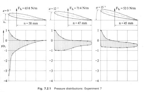Figure 11 – Pressure Distributions at varying angles of attack

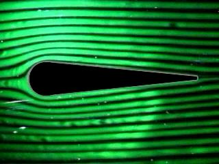
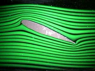
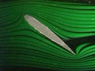
Observe the foil in the smoke tunnel (figure 12) at high angles of attack and note that the flow separates near the leading edge and gives rise to a wide turbulent wake.


figure 12a - Foil in viscous flow at varying angles of attack	figure 12b - Foil of varying thickness in viscous flow

Kutta-Joukowsky Theorem

Now that we have observed that circulation creates lift, how much lift is created? The Kutta-Joukowsky theorem for 2D foils states that the lift force is equal to the circulation times the density times the velocity of the fluid. The minus sign is by convention due to the direction of circulation.

The validity of the Kutta-Joukowsky theorem can be confirmed as follows. Figure 13 shows the velocity distribution around the airfoil at an angle of attack of 6^degrees, calculated from the observed pressure using the Bernoulli equation. To allow for the presence of the boundary layer, these calculated velocities are assumed to apply to a profile lying at an arbitrary distance of 1mm from the airfoil surface and the curves show velocity against the length of this profile, measured from the leading edge. The corresponding circulation is calculated from the circulation equation and from the corresponding lift coefficient. The resulting value C_L = 0.6, is in reasonable agreement with the value C_L = 0.567 calculated from the pressure distribution shown in figure 11.

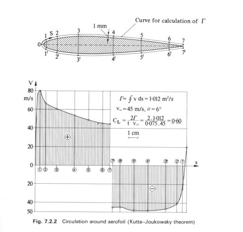Figure 13 – Circulation around airfoil – Kutta-Joukowsky theorem

Please note that all the video material on this page is exclusively the Copyright property of Stanford University and its licensors

References

1- Fluid Mechanics with Engineering Applications - Daugherty

2- A first course in fluid dynamics - Patterson

3- Fluid Mechanics for Engineers - P.S. Bana 1969

4- Fluid Mechanics: A Laboratory Course - Plint/Boswirth

5- Marine Hydrodynamics, J. N. Newman